Category Archives: Statistical analysis

Analysis of parallel temperature data using t-tests

Part 2. Brisbane Airport

Dr Bill Johnston

Using paired and un-paired t-tests to compare long timeseries of data observed in parallel by instruments housed in the same or different Stevenson screens at one site, or in screens located at different sites, is problematic. Part of the problem is that both tests assume that the air being monitored is the control variable. That air inside the screen is spatially and temporally homogeneous, which for a changeable, turbulent medium is not the case.  

Irrespective of whether data are measured on the same day, paired t-tests require the same parcels of air to be monitored by both instruments 100% of the time. As instruments co-located in the same Stevenson screen are in different positions their data cannot be considered ‘paired’ in the sense required by the test. Likewise for instruments in separate screens, and especially if temperature at one site is compared with daily values measured some distance away at another.

As paired t-tests ascribe all variation to subjects (the instruments), and none to the response variable (the air) test outcomes are seriously biased compared to un-paired tests, where variation is ascribed more generally to both the subjects and the response.

The paired t-test compares the mean of the differences between subjects with zero, whereas the un-paired test compares subject means with each other. If the tests find a low probability (P) that that the mean difference is zero, or that subject means are the same, typically less than (P<) 0.05, 5% or 1 in 20, it can be concluded that subjects differ in their response (i.e., the difference is significant). Should probability be less than 0.01 (P<0.01 = 1% or 1 in 100) the between-subject difference is highly significant. However, significance itself does not ensure that the size of difference is meaningful in the overall scheme of things.

Assumptions

All statistical tests are based on underlying assumptions that ensure results are trustworthy and unbiased. The main assumption for is that differences in the case of paired tests, and for unpaired tests, data sequenced within treatment groups are independent meaning that data for one time are not serially correlated with data for other times. As timeseries embed seasonal cycles and in some cases trends, steps must be taken to identify and mitigate autocorrelation prior to undertaking either test.  

A second, but less important assumption for large datasets, is that data are distributed within a bell-shaped normal distribution envelope with most observations clustered around the mean and the remainder diminishing in number towards the tails.

Finally, a problem unique to large datasets is that the denominator in the t-test equation becomes diminishingly small as the number of daily samples increase. Consequently, the t‑statistic becomes exponentially large, together with the likelihood of finding significant differences that are too small to be meaningful. In statistical parlance this is known as Type1 error – the fallacy of declaring significance for differences that do not matter. Such differences could be due to single aberrations or outliers for instance.

A protocol

Using a parallel dataset related to a site move at Townsville airport in December 1994, a protocol has been developed to assist avoiding pitfalls in applying t-tests to timeseries of parallel data. At the outset, an estimate of effect size, determined as the raw data difference divided by the standard deviation (Cohens d) assesses if the difference between instruments/sites is likely to be meaningful. An excel workbook was provided with step-by-step instructions for calculating day-of-year (1-366) averages that define the annual cycle, constructing a look-up table and deducting respective values from data thereby producing de-seasoned anomalies. Anomalies are differenced as an additional variable (Site2 minus Site1, which is the control).

Having prepared the data, graphical analysis of their properties, including autocorrelation function (ACF) plots, daily data distributions, probability density function (PDF) plots, and inspection of anomaly differences assist in determining which data to compare (raw data or anomaly data). The dataset that most closely matches the underlying assumptions of independence and normality should be chosen and where autocorrelation is unavoidable, randomised data subsets offer a way forward. (Randomisation may be done in Excel and subsets of increasing size used in the analysis.)

Most analyses can be undertaken using the freely available statistical application PAST from the University of Oslo: https://www.nhm.uio.no/english/research/resources/past/ Specific stages of the analysis have been referenced to pages in the PAST manual.

The Brisbane Study

The Brisbane study replicates the previous Townsville study, with the aim of showing that protocols are robust. While the Townsville study compared thermometer and automatic weather station maxima measured in 60-litre screens located 172m apart, the Brisbane study compared Tmax for two AWS each with 60-litre screens, 3.2 km apart, increasing the likelihood that site-related differences would be significant.

While the effect size for Brisbane was triflingly small (Cohens d = 0.07), and the difference between data-pairs stabilised at about 940 sub-samples, a significant difference between sites of 0.25oC was found when the number of random sample-pairs exceeded about 1,600. Illustrating the statistical fallacy of excessive sample numbers, differences became significant because the dominator in the test equation (the pooled standard error) declined as sample size increased, not because the difference widened. PDF plots suggested it was not until the effect size exceeded 0.2, that simulated distributions showed a clear separation such that the difference between Series1 and Series2 of 0.62oC could be regarded as both significant and meaningful in the overall scheme of things.

Importantly, the trade-off between significance and effect size is central to avoiding the trap of drawing conclusions based on statistical tests alone.

Dr Bill Johnston

4 June 2023

Two important links – find out more

First Link: The page you have just read is the basic cover story for the full paper. If you are stimulated to find out more, please link through to the full paper – a scientific Report in downloadable pdf format. This Report contains far more detail including photographs, diagrams, graphs and data and will make compelling reading for those truly interested in the issue.

Click here to access a full pdf report containing detailed analysis and graphs

Second Link: This link will take you to a downloadable Excel spreadsheet containing a vast number of data used in researching this paper. The data supports the Full Report.

Click here to download a full Excel data pack containing the data used in this research
Why statistical tests matter

Fake-news, flash-bangs

and why statistical tests matter

Dr Bill Johnston

www.bomwatch.com.au

Main Points

Comparing instruments using paired t-tests, verses unpaired tests on daily data is inappropriate. Failing to verify assumptions, particularly that data are independent (not autocorrelated), and not considering the effect of sample size on significance levels creates illusions that differences between instruments are significant or highly significant when they are not. Using the wrong test and naïvely or bullishly disregarding test assumptions plays to tribalism not trust.

Investigators must justify the tests they use, validate that assumptions are not violated, that differences are meaningful and thereby show their conclusions are sound. 

Discussion

Paired or repeated-measures t-tests are commonly used to determine the effect of an intervention by observing the same subjects before and after (e.g., 10 subjects before and after a treatment). As within-subjects variation is controlled, differences are attributable to the treatment. In contrast, un-paired or independent t‑tests compare the means of two groups of subjects, each having received one of two interventions (10 subjects that received one or no treatment vs. 10 that were treated). As variation between subjects contributes variation to the response, un-paired t-tests are less sensitive than paired tests.

Extended to a timeseries of sequential observations by different instruments (Figure 1), the paired t-test evaluates the probability that the mean of the difference between data-pairs (calculated as the target series minus the control) is zero. If the t‑statistic indicates the mean of the differences is not zero, the alternative hypothesis that the two instruments are different prevails. In this usage, significant means there is a low likelihood, typically less than 0.05, 5% or one in 20, that the mean of the difference equals zero. Should the P-value be less than 0.01, 0.001, or smaller, the difference is regarded as highly significant. Importantly, significant and highly significant are statistical terms that reflect the probability of an effect, not whether the size of an effect is meaningful.

To reiterate, paired tests compare the mean of the difference between instruments with zero, while un-paired t‑tests evaluate whether Tmax measured by each instrument is the same.

While sounding pedantic, the two tests applied to the same data result in strikingly different outcomes, with the paired test more likely to show significance. Close attention to detail and applying the right test is therefore vitally important.

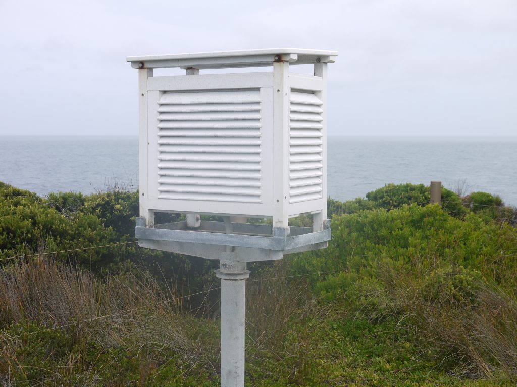
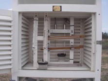
Figure 1. Inside the current 60-litre Stevenson screen at Townsville airport. At the front are dry and wet-bulb thermometers, behind are maximum (mercury) and minimum (alcohol) thermometers, held horizontally to minimise “wind-shake” which can cause them to re-set, and at the rear, which faces north, are dry and wet-bub AWS sensors. Cooled by a small patch of muslin tied by a cotton wick that dips into the water reservoir, wet-bulb depression is used to estimate relative humidity and dew point temperature. (BoM photograph).

Thermometers Vs PRT Probes

Comparisons of thermometers and PRT probes co-located in the same screen, or in different screens, rely on the air being measured each day as the test or control variable, thereby presuming that differences are attributable to instruments. However, visualize conditions in a laboratory verses those in a screen where the response medium is constantly circulating and changing throughout the day at different rates. While differences in the lab are strictly attributable, in a screen, a portion of the instrument response is due to the air being monitored. As shown in Figure 1, instruments that are not accessed each day are more conveniently located behind those that are, thereby resulting in spatial bias. The paired t-test, which apportions all variation to instruments is the wrong test under the circumstances.

Test assumptions are important

The validity of statistical tests depends on assumptions, the most important of which for paired t-tests is that differences at one time are not influenced by differences at previous times. Similarly for unpaired tests where observations within groups cannot be correlated to those previous. Although data should ideally be distributed within a bell-shaped normal-distribution envelope, normality is less important if data are random and numbers of paired observations exceed about 60. Serial dependence or autocorrelation reduces the denominator in the t-test equation, which increases the likelihood of significant outcomes (false positives) and fatally compromises the test.

Primarily caused by seasonal cycles the appropriate adjustment for daily timeseries is to deduct day-of-year averages from respective day-of-year data and conduct the right test on seasonally adjusted anomalies.

Covariables on which the response variable depends are also problematic. These includes heating of the landscape over previous days to weeks, and the effects of rainfall and evaporation that may linger for months and seasons. Removing cycles, understanding the data, using sampling strategies and P-level adjustments so outcomes are not biased may offer solutions.

Significance of differences vs. meaningful differences

A problem of using t-tests on long time series is that as numbers of data-pairs increase, the denominator in the t-test equation, which measures variation in the data, becomes increasingly small. Thus, the ratio of signal (the instrument difference) to noise (the standard error, pooled in the case of un-paired tests) increases. The t‑value consequently becomes exponentially large, the P-level declines to the millionth decimal place and the test finds trifling differences to be highly significant, when they are not meaningful. So, the significance level needs to be considered relative to the size of the effect.

For instance, a highly significant difference that is less than the uncertainty of comparing two observations (±0.6oC) could be an aberration caused by averaging beyond the precision of the experiment (i.e., averaging imprecise data to two, three or more decimal places).

The ratio of the difference to the average variation in the data [i.e., (PRTaverage minus thermometeraverage) divided by the average standard deviation], which is known as Cohens d, or the effect size, also provides a first-cut empirical measure that can be calculated from data summaries to guide subsequent analysis.

Cohens d indicates whether a difference is likely to be negligible (less than 0.2 SD units), small (>0.2), medium (>0.5) or large (<0.8), which identifies traps to avoid, particularly the trap of unduly weighting significance levels that are unimportant in the overall scheme of things.

The Townsville case study

T-tests of raw data were invalidated by autocorrelation while those involving seasonally adjusted anomalies showed no difference. Randomly sampled raw data showed significance levels depended on sample size not the difference itself, thus exposing the fallacy of using t‑tests on excessively large numbers of data-pairs. Irrespective of the tests, the effect size calculated from the data summary of 0.12 SD units is trivial and not important.     

Conclusions

Using paired verse unpaired t-tests on timeseries of daily data inappropriately, not verifying assumptions, and not assessing the effect size of the outcome creates division and undermines trust. As illustrated by Townsville, it also distracts from real issues. Using the wrong test and naïvely or bullishly disregarding test assumptions plays to tribalism not trust.

A protocol is advanced whereby autocorrelation and effect size are examined at the outset. It is imperative that this be carried out before undertaking t-tests of daily temperatures measured in-parallel by different instruments.

The overarching fatal error is using invalid tests to create headlines and ruckus about thin-things that make no difference, while ignoring thick-things that would impact markedly on the global warming debate.

Two important links – find out more

First Link: The page you have just read is the basic cover story for the full paper. If you are stimulated to find out more, please link through to the full paper – a scientific Report in downloadable pdf format. This Report contains far more detail including photographs, diagrams, graphs and data and will make compelling reading for those truly interested in the issue.

Click here to download the full paper Statistical_Tests_TownsvilleCaseStudy_03June23

Second Link: This link will take you to a downloadable Excel spreadsheet containing a vast number of data points related to the Townsville Case Study and which were used in the analysis of the Full Report.

Click here to access the full data used in this post Statistical tests Townsville_DataPackage

Day/Night temperature spread fails to confirm IPCC prediction

By David Mason-Jones, 

Research by Dr. Lindsay Moore

The work of citizen scientist, Dr. Lindsay Moore, has failed to confirm an important IPCC prediction about what will happen to the spread between maximum and minimum temperatures due to the Enhanced Greenhouse Effect. The IPCC’s position is that this spread will narrow as a result of global warming.

Moore’s work focuses on the remote weather station at Giles in Western Australia and run by Australia’s peak weather monitoring body, the Bureau of Meteorology (BoM).

Why Giles? 

Giles is the most remote weather station in mainland Australia and its isolation in a desert makes it an ideal place to study the issue of temperature spread. It is virtually in the middle of the Continent.It is far from influencing factors such as Urban Heat Island effect, land use changes, encroachment by shading vegetation, shading by buildings and so on, that can potentially corrupt the data. Humidity is usually low and stable and it is far from the sea. In addition, as a sign of its importance in the BoM network, Giles is permanently staffed.

As stated, the IPCC hypothesis is that the ‘gap’ will become steadily smaller as the Enhanced Greenhouse Effect takes hold. As temperature rises the gap will narrow and this will result in an increase in average temperature, so says the IPCC.

Moore’s research indicates that this is just not happening at this showcase BoM site. It may be happening elsewhere, and this needs to be tested in each case against the range of all data-corrupting effects, but it is not happening at Giles.

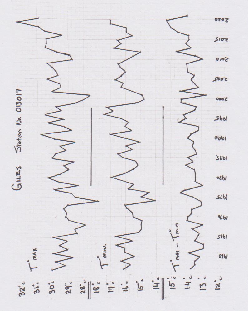
Notes about the graphs. The top plot line shows the average Tmax for each year – that is, the average maximum daytime temperature. The middle plot shows the average Tmin for each year – that is, the average minimum night time temperature.

The lower plot shows the result of the calculation Tmax-Tmin. In laypersons’ terms it is the result you get when you subtract the average yearly minimum temperature from the average yearly maximum temperature. If the IPCC hypothesis is valid, then the lower plot line should be falling steadily through the years because, according to the IPCC, more carbon dioxide in the atmosphere should make nights warmer. Hence, according to the IPCC’s hypothesis, the gap between Tmax and Tmin will become smaller – ie the gap will narrow. But the plot line does not show this.

The IPCC’s reasoning for its narrowing prediction is that global warming will be driven more by a general rise in minimum temps that it will be by a general rise in maximums. This is not my assertion, nor is it Dr. Moore’s, it is the assertion of the IPCC and can be found in the IPCC’s AR4 Report. 

Dr. Moore states, “In the AR4 report the IPCC claims that elevated CO2 levels trap heat, specifically the long wave radiation escaping to space.

“As a result of this the IPCC states at page 750 that, ‘almost everywhere night time temperatures increase more than day time temperatures, that decrease in number of frost days are projected over time, and that temperatures over land will be approximately twice average Global temp rise,” he says citing page 749 of the AR4 report. 

So where can we go to find evidence that the IPCC assertion of a narrowing spread of Tmax-Tmin is either happening or not happening? Giles is a great start point. Can we use the BoM’s own publicly available data to either confirm, or disprove, the narrowing prediction? The short answer is – Yes we can.

But, before we all get too excited about the result Dr. Moore has found, we need to recognise the limitation that this is just one site and, to the cautious scientific mind, may still be subject to some bizarre influence that somehow skews the result away from the IPCC prediction. If anyone can suggest what viable contenders for ‘bizarre influences’ might be at Giles we would welcome them in the comments section of this post. 

The caution validly exercised by the rigorous scientific mind can be validly balanced by the fact that Giles is a premier, permanently staffed and credible site. The station was also set up with great care, and for very specific scientific purposes, in the days of the Cold War as part of the British nuclear test program in Australia in the 1950’s. It was also important in supplying timely and accurate meteorological data for rocket launches from the Woomera Rocket Range in South Australia in the development of the Bluestreak Rocket as part of the British/Australian space program. This range extended almost all the way across Australia from the launching site at Woomera to the arid North West of Western Australia.

In the early years there were several other weather monitoring stations along the track of the range. Such has been the care and precision of the operation of the station that Giles has the characteristics of a controlled experiment. 

Dr. Moore states, “Giles is arguably the best site in the World because of its position and the accuracy and reliability of its records which is a constant recognised problem in many sites. Data is freely available on the BoM website for this site.”

With regard to the site validly having the nature of a controlled experiment, something about the method of analysis is also notable. The novel adoption of deriving the spread Tmax-Tmin  by doing it on a daily basis neatly avoids meta data issues that have plagued the reliability of data from other stations and sometimes skewed results from other supposedly reliable observation sites.

“I would argue that the only change in environmental conditions over the life of this station is the increase in CO2 from 280 to 410 ppm,” he says.

“In effect this is, I suggest, a controlled experiment with the only identifiable variable input being CO2 concentration,” he says.  

The conclusion reached by Dr. Moore is that an examination of the historical records for this site by accessing the same data through the BoM website unequivocally shows NO significant reduction in Tmax-Tmin. It also shows no rise in Tmin. Anyone can research this data on the Bureau of Meteorology website as it is not paywalled. It is truly sound data from a government authority for the unrestricted attention of citizens and other researchers.  

Dr. Moore concludes, “The logical interpretation of this observation is that, notwithstanding any other unidentified temperature influencing factor, the Enhanced Greenhouse Effect due to elevated CO2 had no discernible effect on temperature spread at this site. And, by inference, any other site.”

He further states, “On the basis of the observations I have made, there can be no climate emergency due to rising CO2 levels, whatever the cause of the rise. To claim so is just scaremongering.

“Any serious climate scientist must surely be aware of such basic facts yet, despite following the science for many years, I have never seen any discussion on this specific approach,” he says.

Finally, Dr. Moore poses a few questions and makes some pertinent points:

He asks, “Can anyone explain, given the current state of the science why there is no rise in minimum temperatures (raw) or, more importantly, no reduction in Tmax-Tmin spread, over the last 65 years of records despite a significant rise in CO2 levels at Giles (280-410ppm) as projected by the IPCC in their AR4 report?” He notes that other published research indicates similar temperature profiles in the whole of the central Australian region as well as similarly qualified North American and World sites.

Seeking further input, he asks, “Can anyone provide specific data that demonstrates that elevated CO2 levels actually do increase Tmin as predicted by the IPCC?” And further, “Has there been a reduction in frost days in pristine sites as predicted by the IPCC?”

On a search for more information, he queries, “Can anyone explain why the CSIRO ‘State of the Climate’ statement (2020) says that Australian average temperatures have risen by more than 1 deg C since 1950 when, clearly, there has been no such rise at this pristine site?” With regard to this question, he notes that Giles should surely be the ‘go to’ reference site in the Australian Continent.

Again he tries to untangle the web of conflicting assertions by reputedly credible scientific organisations. He notes that, according to the IPCC rising average temperatures are attributable to rise in minimum temperatures. For the CSIRO State of the Climate statement to be consistent with this, it would necessitate a rise of around 2 deg C in Tmin. But, at Giles, there was zero rise. He also notes that, according to the IPCC, temperature rises over land should be double World average temperature rises. But he can see no data to support this. 

Dr. Moore’s final conclusion: “Through examination of over 65 years of data at Giles it can be demonstrated that, in the absence of any other identifiable temperature forcing, the influence of the Enhanced Greenhouse Effect at this site appears to be zero,” he says. “Not even a little bit!” 

David Mason-Jones is a freelance journalist of many years’ experience. He publishes the website www.bomwatch.com.au

Dr. Lindsay Moore, BVSC. For approaching 50 years Lindsay Moore  has operated a successful veterinary business in a rural setting in the Australian State of Victoria. His veterinary expertise is in the field of large animals and he is involved with sophisticated techniques such as embryo transfer. Over the years he has seen several major instances in veterinary science where something that was once accepted on apparently reasonable grounds, and adopted in the industry, has later been proven to be incorrect. He is aware that this phenomenon is not only confined to the field of Veterinary Science but is happens in other scientific fields as well. The lesson he has taken from this is that science needs to advance with caution and that knee-jerk assumptions about ‘the science is settled’ can lead to significant mistakes. Having become aware of this problem in science he has become concerned about how science is conducted and how it is used. He has been interested in the global warming issue for around 20 years.   

General link to Bureau of Meteorology website is www.bom.gov.au

About

Welcome to BomWatch.com.au a site dedicated to examining Australia’s Bureau of Meteorology, climate science and the climate of Australia. The site presents a straight-down-the-line understanding of climate (and sea level) data and objective and dispassionate analysis of claims and counter-claims about trend and change.

BomWatch delves deeply into the way in which data has been collected, the equipment that has been used, the standard of site maintenance and the effect of site changes and moves.

Dr. Bill Johnston is a former senior research scientist with the NSW Department of Natural Resources (abolished in April 2007); which in previous guises included the Soil Conservation Service of NSW; the NSW Water Conservation and Irrigation Commission; NSW Department of Planning and Department of Lands. Like other NSW natural resource agencies that conducted research as a core activity including NSW Agriculture and the National Parks and Wildlife Service, research services were mostly disbanded or dispersed to the university sector from about 2005.

BomWatch.com.au is dedicated to analysing climate statistics to the highest standard of statistical analysis

Daily weather observations undertaken by staff at the Soil Conservation Service’s six research centres at Wagga Wagga, Cowra, Wellington, Scone, Gunnedah and Inverell were reported to the Bureau of Meteorology. Bill’s main fields of interest have been agronomy, soil science, hydrology (catchment processes) and descriptive climatology and he has maintained a keen interest in the history of weather stations and climate data. Bill gained a Batchelor of Science in Agriculture from the University of New England in 1971, Master of Science from Macquarie University in 1985 and Doctor of Philosophy from the University of Western Sydney in 2002 and he is a member of the Australian Meteorological and Oceanographic Society (AMOS).

Bill receives no grants or financial support or incentives from any source.

BomWatch accesses raw data from archives in Australia so that the most authentic original source-information can be used in our analysis.

How BomWatch operates

BomWatch is not intended to be a blog per se, but rather a repository for analyses and downloadable reports relating to specific datasets or issues, which will be posted irregularly so they are available in the public domain and can be referenced to the site. Issues of clarification, suggestions or additional insights will be welcome.   

The areas of greatest concern are:

  • Questions about data quality and data homogenisation (is data fit for purpose?)
  • Issues related to metadata (is metadata accurate?)
  • Whether stories about datasets consistent and justified (are previous claims and analyses replicable?)

Some basic principles

Much is said about the so-called scientific method of acquiring knowledge by experimentation, deduction and testing hypothesis using empirical data. According to Wikipedia the scientific method involves careful observation, rigorous scepticism about what is observed … formulating hypothesis … testing and refinement etc. (see https://en.wikipedia.org/wiki/Scientific_method).

The problem for climate scientists is that data were not collected at the outset for measuring trends and changes, but rather to satisfy other needs and interests of the time. For instance, temperature, rainfall and relative humidity were initially observed to describe and classify local weather. The state of the tide was important for avoiding in-port hazards and risks and for navigation – ships would leave port on a falling tide for example. Surface air-pressure forecasted wind strength and direction and warned of atmospheric disturbances; while at airports, temperature and relative humidity critically affected aircraft performance on takeoff and landing.

Commencing in the early 1990s the ‘experiment’, which aimed to detect trends and changes in the climate, has been bolted-on to datasets that may not be fit for purpose. Further, many scientists have no first-hand experience of how data were observed and other nuances that might affect their interpretation. Also since about 2015, various data arrive every 10 or 30 minutes on spreadsheets, to newsrooms and television feeds largely without human intervention – there is no backup paper record and no way to certify those numbers accurately portray what is going-on.

For historic datasets, present-day climate scientists had no input into the design of the experiment from which their data are drawn and in most cases information about the state of the instruments and conditions that affected observations are obscure.

Finally, climate time-series represent a special class of data for which usual statistical routines may not be valid. For instance, if data are not free of effects such as site and instrument changes, naïvely determined trend might be spuriously attributed to the climate when in fact it results from inadequate control of the data-generating process: the site may have deteriorated for example or ‘trend’ may be due to construction of a road or building nearby. It is a significant problem that site-change impacts are confounded with the variable of interest (i.e. there are potentially two signals, one overlaid on the other).

What is an investigation and what constitutes proof?

 The objective approach to investigating a problem is to challenge the straw-horse argument that there is NO change, NO link between variables, NO trend; everything is the same. In other words, test the hypothesis that data consist of random numbers or as is the case in a court of law, the person in the dock is unrelated to the crime. The task of an investigator is to open-handedly test that case. Statistically called a NULL hypothesis, the question is evaluated using probability theory, essentially: what is the probability that the NULL hypothesis is true?

In law a person is innocent until proven guilty and a jury holding a majority view of the available evidence decides ‘proof’. However, as evidence may be incomplete, contaminated or contested the person is not necessarily totally innocent –he or she is simply not guilty.

In a similar vein, statistical proof is based on the probability that data don’t fit a mathematical construct that would be the case if the NULL hypothesis were true. As a rule-of-thumb if there is less than (<) a 5% probability (stated as P < 0.05) that that a NULL hypothesis is supported, it is rejected in favour of the alternative. Where the NULL is rejected the alternative is referred to as significant. Thus in most cases ‘significant’ refers to a low P level. For example, if the test for zero-slope finds P is less than 0.05, the NULL is rejected at that probability level, and trend is ‘significant’. In contrast if P >0.05, trend is not different to zero-trend; inferring there is less than 1 in 20 chance that trend (which measures the association between variables) is not due to chance.

Combined with an independent investigative approach BomWatch relies on statistical inference to draw conclusions about data. Thus the concepts briefly outlined above are an important part of the overall theme. 

Using the air photo archives available in Australia, Dr Bill Johnston has carried out accurate and revealing information about how site changes have been made and how these have affected the integrity of the data record.